Machine Learning
Machine Learning
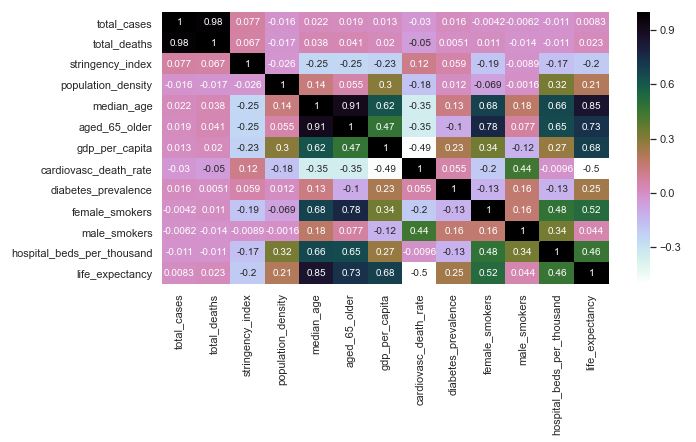
Heatmap for the Correlation Matrix
This heatmap shows the correlation between the different categories. This allows us to see how the different categories may effect each other. We can observe that median_age, aged_65_older and aged_70_older are correlated. We will include only median_age and aged_65_older in our model to avoid noise.
Linear Regression
We performed a linear regression on our EU data frame to understand the impact of GDP, demographic factors like age, prevalence of smoking, life expectancy, median age, location total cases.
The intercept term of the linear model: 2243.888492529553
Linear Regression Coefficients are as below:
| Coefficients | |
|---|---|
| total_cases | 4.388124e+03 |
| stringency_index | 4.041565e+02 |
| population_density | -7.639171e+15 |
| median_age | 1.145649e+16 |
| aged_65_older | -9.617242e+15 |
| gdp_per_capita | 2.845609e+16 |
| cardiovasc_death_rate | 2.546675e+16 |
| diabetes_prevalence | 1.111645e+16 |
| female_smokers | 1.107000e+16 |
| male_smokers | 4.598792e+15 |
| hospital_beds_per_thousand | 2.914445e+16 |
| life_expectancy | -2.018291e+16 |
| iso_code_AND | 1.677666e+16 |
| iso_code_AUT | 1.008480e+16 |
| iso_code_BEL | -2.479658e+16 |
| iso_code_BGR | -1.401767e+16 |
| iso_code_BIH | -3.326751e+16 |
| iso_code_BLR | -2.110048e+16 |
| iso_code_CHE | -3.052661e+15 |
| iso_code_CYP | -1.225351e+16 |
| iso_code_CZE | -1.263972e+15 |
| iso_code_DEU | 7.723661e+15 |
| iso_code_DNK | 2.689768e+16 |
| iso_code_ESP | 2.775221e+15 |
| iso_code_EST | 4.449207e+15 |
| iso_code_FIN | 6.387662e+15 |
| iso_code_FRA | 5.909560e+16 |
| iso_code_FRO | 1.350117e+16 |
| iso_code_GBR | 1.100902e+16 |
| iso_code_GGY | -1.286488e+16 |
| iso_code_GIB | 1.040587e+16 |
| iso_code_GRC | -6.008871e+14 |
| iso_code_HRV | -9.216104e+15 |
| iso_code_HUN | -1.994166e+16 |
| iso_code_IMN | 1.659487e+16 |
| iso_code_IRL | -1.119291e+16 |
| iso_code_ISL | 6.475450e+15 |
| iso_code_ITA | -2.739907e+16 |
| iso_code_JEY | 3.690339e+15 |
| iso_code_LIE | 3.272328e+14 |
| iso_code_LTU | -1.701523e+16 |
| iso_code_LUX | -2.166666e+16 |
| iso_code_LVA | 5.074342e+15 |
| iso_code_MCO | 1.041756e+15 |
| iso_code_MDA | -1.326413e+16 |
| iso_code_MKD | -1.458366e+16 |
| iso_code_MLT | 5.813585e+15 |
| iso_code_MNE | -2.075621e+16 |
| iso_code_NLD | -2.445927e+16 |
| iso_code_NOR | -6.922632e+15 |
| iso_code_OWID_KOS | -2.415548e+16 |
| iso_code_POL | -2.412902e+16 |
| iso_code_PRT | -2.519373e+16 |
| iso_code_ROU | -2.036722e+15 |
| iso_code_RUS | -2.596940e+16 |
| iso_code_SMR | 3.837194e+16 |
| iso_code_SRB | -1.672350e+16 |
| iso_code_SVK | 1.518220e+15 |
| iso_code_SVN | -1.782923e+16 |
| iso_code_SWE | 3.207623e+15 |
| iso_code_UKR | -9.536771e+14 |
| iso_code_VAT | -2.010495e+15 |
| location_Andorra | -1.694448e+16 |
| location_Austria | -2.107024e+16 |
| location_Belarus | -7.335600e+14 |
| location_Belgium | 2.307448e+16 |
| location_Bosnia and Herzegovina | 2.486882e+16 |
| location_Bulgaria | -1.359825e+15 |
| location_Croatia | 1.383471e+14 |
| location_Cyprus | 1.179733e+16 |
| location_Czech Republic | -1.031157e+16 |
| location_Denmark | -2.350112e+16 |
| location_Estonia | -8.848710e+15 |
| location_Faeroe Islands | -1.403089e+16 |
| location_Finland | -2.233834e+15 |
| location_France | -6.015327e+16 |
| location_Germany | -2.255030e+16 |
| location_Gibraltar | -1.034263e+16 |
| location_Greece | -1.232976e+15 |
| location_Guernsey | 1.283442e+16 |
| location_Hungary | 7.394707e+15 |
| location_Iceland | 1.260433e+15 |
| location_Ireland | 9.888678e+15 |
| location_Isle of Man | -1.655653e+16 |
| location_Italy | 3.329812e+16 |
| location_Jersey | -3.721587e+15 |
| location_Kosovo | 2.901669e+16 |
| location_Latvia | -1.650324e+16 |
| location_Liechtenstein | 2.428077e+15 |
| location_Lithuania | 3.960924e+15 |
| location_Luxembourg | 9.274371e+15 |
| location_Macedonia | 5.159152e+15 |
| location_Malta | -7.060992e+15 |
| location_Moldova | 5.215677e+15 |
| location_Monaco | -5.972042e+15 |
| location_Montenegro | 7.535881e+15 |
| location_Netherlands | 2.518425e+16 |
| location_Norway | 5.814110e+15 |
| location_Poland | 1.731636e+16 |
| location_Portugal | 2.693640e+16 |
| location_Romania | -1.710978e+16 |
| location_Russia | 2.001379e+15 |
| location_San Marino | -3.982231e+16 |
| location_Serbia | -4.298116e+14 |
| location_Slovakia | -1.209923e+16 |
| location_Slovenia | 1.704641e+16 |
| location_Spain | -4.683184e+14 |
| location_Sweden | 3.958107e+15 |
| location_Switzerland | 5.861035e+14 |
| location_Ukraine | -1.873240e+16 |
| location_United Kingdom | -3.976763e+15 |
| location_Vatican | -2.218792e+15 |
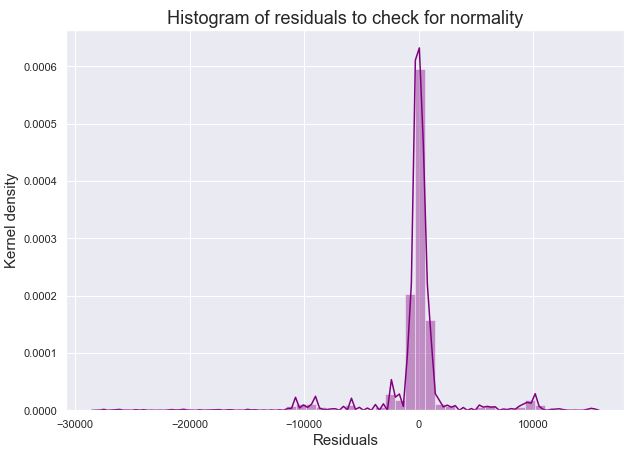
The model accuracy came as 70.5% from this. To check if this model is valid we plotted the residuals for normality and residuals versus predicted for homoscedasticity.
Below plot shows us that the residuals though might seem like normally distributed but narrower plot are not normally distributed.
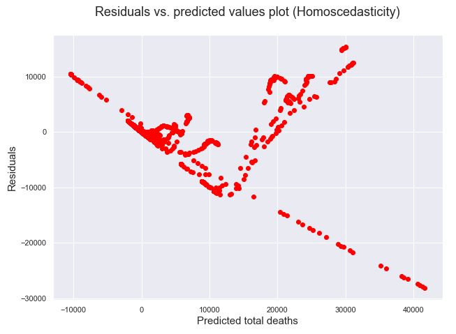
From below residuals vs predicted plot we can observe that this data set is not good for a linear regression model.
Decision Tree Model
We also ran the decision tree model and observed it performs better once tuned with GridSearchCV to find the best possible parameters to understand the total deaths with GDP and age parameters for different locations across Europe. Below are the results which shows that the model is well tuned to predict the total deaths very closely:
Train score: 0.924
Test score: 0.918
DecisionTreeRegressor(criterion='mse', max_depth=3, max_features=None,
    max_leaf_nodes=4, min_impurity_decrease=0.0,
    min_impurity_split=None, min_samples_leaf=1,
    min_samples_split=2, min_weight_fraction_leaf=0.0,
    presort=False, random_state=100, splitter='best')